
6
Número 16 Vol. 2 (2016)
ATMOSPHERIC TRANSMISIVITY: A MODEL
COMPARISON FOR EQUATORIAL ANDEAN
HIGHLANDS ZONE
Cristina Ramos
1 2
, *Natalia Pérez
2
, Geovanna Villacreses
1
, Diego Vaca
1
, Estefanía Chávez
2
, and
Mario Pérez
2
1
Instituto Nacional de Eciencia Energética y Energía Renovable, Quito (Ecuador)
2
Escuela Superior Politécnica de Chimborazo - Escuelas de Física Matemática y Ciencias Quími-
cas, Riobamba (Ecuador). *natalia.perezlondo@gmail.com
R
esumen
A
bstract
Ecuador is a South American country divided by the Equator. It is bordered by Colombia to the
North, Peru to the East and South, and bounded on the West by the Pacic Ocean. Due to its loca-
tion, Ecuador experiences very little variation in sunshine duration and very intense solar radiation.
Moreover, about one third of the country is located at higher altitudes because of the presence of the
Andes Mountain range, which means that those places receive higher solar radiation compared with
lower regions of the country. However, there is not enough meteorological time series available for
the entire region, especially for solar radiation. Nevertheless, in Riobamba (a city at 2750 m.a.s.l.),
total solar radiation has been measured since 2007 with automatic meteorological stations and total
sunshine hours, daily temperatures, precipitation, and wind speed since 1975 with a mechanical wea-
ther station. This data were used to calculate coefcients of atmospheric transmissivity by means of
six well-known models: Prescott, Hargreaves, Garcia, Bristow–Campbell, Hunt, Richardson Reddy.
The results show that the sunshine hour’s model obtained the best performance among all the six
models, indicating that this model could be used to estimate the incident solar radiation in the High
Andean equatorial zone and to impute the missing data of global radiation in the zone. If data of
sunshine hours is not available, the second best model uses temperatures and wind speed.
Keywords:Solar radiation, High Andean equatorial zone, model application.
Ecuador es un país ubicado en América del Sur dividido por la línea Ecuatorial. Al norte está limitado
por Colombia, al sur y al este por Perú y al oeste por el Océano Pacíco. Debido a su localización,
Ecuador percibe una pequeña variación en la duración de las horas de sol e intensa radiación solar.
Además, alrededor de un tercio del país está localizado en las partes más altas debido a la presen-
cia de la cordillera de los Andes lo cual signica que todos estos lugares reciben una alta radiación
solar comparada con las regiones más bajas del país. Sin embargo, no existe una suciente cantidad
de series de datos meteorológicos disponibles de toda la región, especialmente de radiación solar.
Favorablemente en Riobamba (una ciudad a 2750 m.s.n.m), los datos de radiación solar han sido
medidos por una estación meteorológica automática desde el 2007 y los datos de horas de sol, tem-
peraturas diarias, precipitación y velocidad de viento han sido medidos desde 1975 por una estación
meteorológica manual. Estos datos han sido usados para calcular los coecientes de transmisibilidad
atmosférica de seis modelos conocidos: Prescott, Hargreaves, Garcia, Bristow–Campbell, Hunt, Ri-
chardson Reddy. Los resultados muestran que el modelo basado en las horas de sol ha obtenido el
mejor rendimiento de los seis modelos, indicando que este modelo puede ser utilizado para estimar
la radiación solar incidente en la Zona Ecuatorial Alto Andino y reemplazar los datos faltantes de la
radiación solar en la zona. Si los datos de horas de sol no están disponibles, el siguiente mejor mode-
lo está basado en temperaturas y velocidad de viento.
Palabras claves: Radiación solar, zona ecuatorial alta andina, aplicación de modelo.
Revista Cientíca
ISSN 1390-5740
ISSN 2477-9105

7
1. INTRODUCTION
Using solar technologies could be very
important for Ecuador since its geogra-
phical location and the presence of the
Andes Mountains makes that the solar
radiation is stronger than many other lo-
cations worldwide. In spite of their im-
portance, solar radiation measurements
in Ecuador are rare and infrequent,
mainly due to the cost of specialized
equipment and lack of trained personal.
In the existent meteorological stations,
the main problem is that the data is fre-
quently lost because the equipment is not
frequently maintained and the personal
in charge of taking the measurements is
not properly trained. For this reason, it is
important to perform statistical analysis
to have a trustworthy database (1).
Many models has been developed to
estimate solar radiation by using other
(more common) meteorological varia-
bles such as sunshine duration hours,
minimum and maximum air temperatu-
res, precipitation and wind speed (2,3,4).
Describes work global solar radiation
covering a wide range of geographical
and climate conditions; but there is not
data over Ecuador.
The main objective of this work is to de-
termine the most appropriate empirical
coefcients that are used in the afore-
mentioned models so that be possible to
impute the missing solar radiation data
in the databases.
2. METHODS
2.1 Data
Riobamba is a city situated in the cen-
tral part of Ecuador at latitude 1º 40’ 28’’
South, longitude 78º 38’ 54’’ West and
2750 m.a.s.l. An automatic meteorolo-
gical station was installed and operated
in this city between June 2007 and De-
To detect the presence of multi-variant outliers, the mini-
mum covariance determinant estimator was used. It helps
to the detection of masked outliers (1). A similar solution
was proposed by Peña and Prieto (5); in this method, the
data is projected in specific directions so that they have
high probability of showing outliers. On the other hand,
the coefficient of kurtosis is an indicator of the presence
of small groups of outliers; for this reason, the directions
where the projected points have maximum and minimum
kurtosis were calculated. Then, in these directions, all the
values in all the directions of maximum and minimum
kurtosis are tested with eq. 1. If the values surpass the
value of 5, they are considered suspects of being outliers.
Once these suspects were identified, a vector of means
cember 2012; however, the pyrometer worked until April
2012. The station was registering and recording different
parameters such as temperature, relative humidity, wind
speed, atmospheric pressure and daily average total so-
lar radiation. On the other hand, the National Meteoro-
logical Institute has installed a meteorological station in
the same city and it has provided the daily total hours of
sunshine, maximum daily temperature, minimum daily
temperature, and other parameters for the same period
of time.
The meteorological data was obtained using an automa-
tic station located at latitude 1º 39’ 17’’ South, longitude
78º 49’ 39’’ West, and 2820 m.a.s.l. The available sensors
are: pyrometer (Li-Co #LI-200SA) with certicate of ca-
libration y and error of 5%., thermometer (NGR #110S),
anemometer (NGR #40C) and pluviometer (Rain Gauge
Tipping Bucket). The average values are stored every 10
minutes in a data logger NRG Symphonie. About 950
meters from this station, it is located a manual meteoro-
logical station at latitude 1º 39’ 3’’ South, longitude 78º
41’ 7’’ West, 2840 m.a.s.l. This station has a sunshine du-
ration sensor Campbell-Stokes, which data is registered
physically.
2.2. Detection of outliers
To detect the presence of mono-variant outliers in the
data, it was performed a descriptive analysis using gra-
phics and a robust standardization using the median,
which is an estimator of the central position of the data
and the MEDA, which is a robust estimator of the disper-
sion. This calculation was performed using eq.1.
Ramos,Pérez N,Villacreses,Vaca,Chavez,Pérez M.
xmed x
MEDA x
or
i
−
()
()
>
45
��

8
Número 16 Vol. 2 (2016)
Once the distances of Mahalanobis were obtained for
every suspect data, they were ordered from the minor va-
lue to the major value and they were tested to check if
they can be incorporated to the main group of data of if
they are separated, using a multi-variant inference that
can be found in Peña and Prieto (5).
2.3. Extraterrestrial radiation models.
To calculate the extraterrestrial solar radiation, the an-
gular movement of the Sun observed on the sky was
analyzed. For this purpose, it is necessary to deduct the
solar hour in function of the local hour; the solar noon
is considered when the Sun passes over the observer´s
meridian. In addition, two corrections to the hour where
performed: the rst one consisted in subtracting four mi-
nutes for every degree of difference between the standard
meridian of the country (-78.7°) and the meridian of pla-
ce that is being analyzed (-75°). The second correction
corresponds to the perturbations in Earth´s rate of rota-
tion (3,7).
The extraterrestrial solar radiation can be calculated with
eq. 3 and eq. 4.
Where:
θ
z
is the zenith angle, which determines the position of
the sun with respect to a vertical line.
and a matrix of variances and co-variances of clean data
were calculated in order to compute the distances of Ma-
halanobis of the suspected data, using eq.2. (1,6).
is the latitude of the place. In this
work -1.65°.
is the solar declination, which deter-
mines the angular position of the Sun at
noon with respect to the horizontal pla-
ne.
2.4.1. Hours of sunshine models.
In this work, the equation proposed by
Prescott (eq. 8) was used. The variables
are: Ho as the total calculated extrate-
rrestrial irradiation, H as the incident
irradiation, n as the effective sunshi-
ne hours, N as the theoretical sunshine
hours, and a and b as the empirical coe-
fcients (2, 8).
It is important to mention that theoreti-
cal sunshine hours changes according to
the place and the day of the year. In this
work, it is calculated with eq. 9.
2.4.2. Maximum and minimum tempera-
ture models
To use the maximum and minimum tem-
peratures, three models were applied:
one proposed by Hargreaves (eq. 10) in
1982, another proposed by García (eq.
11) in 1994, and one proposed by Bris-
tow Campbell (eq. 12). (2,9). All these
models use ∆T as the difference between
the maximum and minimum temperatu-
res. It is worth to mention that eq.11 in-
cludes sunshine hours
2.4.3 Models based on temperatures,
precipitation, and wind speed.
To improve the estimation of the solar
radiation based in temperatures, it has
been established that models can be mo-
Where:
Gon is the extraterrestrial solar irradiation.
Gsc is the solar constant.
n’ is the number of the day of the year (1 to 365).
2.4. Estimation of solar radiation models
In order to apply the models to estimate the incident so-
lar extraterrestrial radiation on earth, it is necessary to
calculate the theoretical incident extraterrestrial radiation
(Ho), using eq. 5, eq. 6 and eq. 7.
Dx xxxS xx
Ri RiRR
iR
21
−
()
= −
()
−
()
−
��
� �
'
GG BB B
on sc
= + ++ +1 000110 0 34221 0 001280 0 000719 200..cos. .cos .se
n0
00077 2sen B
()
Bn
= +
()
'1
360
365
HG
oo
nz
= (cos )
θ
cos�sinsin coscos cos
θφδφδω
z
= +
Where:
is the zenith angle, which determines the position of
the sun with respect to a vertical line.
θ
z
φ
δ
H
H
ab
n
N
0
= +
N = − ∅
()
−
2
15
1
costan tan
δ
0
05
H
H
abt=+∆
.
0
1
H
H
abT
BB
c
B
=−−
()
exp ∆
0
1
H
H
abT
BB
c
B
=−−
()
exp ∆
δ
≠
=
−+−
180
0 006918 0 399912 0 070257 0 00675..Cos( ). Sin( ).BB882
0 000907 20002697 3000148 3
Cos( )
.Sin() .Cos() .Sin()
B
BBB
+
−+
Revista Cientíca
ISSN 1390-5740
ISSN 2477-9105

9
died by adding other variables such as
precipitation or wind speed. The model
proposed by Hunt, based in extreme
temperatures and precipitation (eq. 13),
and the model proposed by Richardson
– Reddy (10), that incorporates wind
speed (eq. 14) have been used in this
work.
Where:
are empirical coe-
fcients obtained from a multiple lineal
regression.
Tmax is the maximum temperature °C.
PR is the precipitation in mm.
Where:
are empirical coe-
fcients obtained from a multiple lineal
regression, Ws is the wind speed in m/s.
2.4.4 Models based on satellite images.
Another method that was tried was to
use simple correlations between global
solar radiation and variables measured
with satellites. Two sources of data were
analyzed. The rst one is the GOES
weather satellite which provides infor-
mation of ve spectral bands, including
near infrared and water vapor (11). The
spatial resolution of this data goes from
one kilometer to four kilometers. On the
other hand, the satellites Terra and Aqua
are equipped with a Moderate-Resolu-
tion Imaging Spectroradiometer (MO-
DIS) that captures data in 35 spectral
bands (12). The spatial resolution is 250
meters. For its better spatial resolution,
it was decided to use information from
the MODIS sensor.
The variable selected for to calculate the
simple correlations was the Normalized
Difference Vegetation Index (NDVI),
which is indicator used to estimate the
quantity, quality and development of
vegetation, based on the reection and emission of so-
lar radiation on plants (13). Although the vegetation is
affected by variables such as altitude, precipitation rate,
among others, it has a strong relation with solar radiation.
Then, using monthly averages of solar radiation mea-
sured on eld, and coupling them with monthly avera-
ges of NDVI, obtained from satellite images, a simple
correlation was found to deduct an equation that allows
estimating radiation in un-instrumented places.
3. RESULTS
3.1. Data
From the complete universe of data, for the calculation
of the models the years 2009, 2010 and 2011 were used,
which had to correspond to 1095 registers; however, be-
cause of damaged equipment, maintenance and maxi-
mum capacity of storing, the available data was 75%
approximately. It is important to mention that for all the
statistical analyses to be valid, the data must comply with
the assumption that they have a multi- variant normal
distribution. In this case, this assumption was valid for
years 2009 and 2010. For 2011, the data has mono-va-
riant normal distribution. This means that all the analyses
performed to detect the outliers were valid. On the other
hand, the validation of the models was performed with
data taken from the years 2007, 2008 and 2012, which
represents 33% of the whole registers.
3.2. Detection of outliers.
With the mono-variant and multi-variant techniques for
the detection of outliers, the number of suspected data
was 34. Later, calculating the distances of Mahalanobis,
that has a Chi-squared distribution with 5 degrees of free-
dom, and using multi-variant inference, it was veried
that the whole group of suspects are outliers; consequent-
ly, these registers were not used for the calculations.
3.3. Models for estimation of solar radiation.
Figures from g.1 to g. 3 show the plots of the universe
of registers that were used for the calculation of the em-
pirical coefcients.
Ramos,Pérez N,Villacreses,Vaca,Chavez,Pérez M.
abcd e
HHH
HH
,� ,� ,� � ,� �
H
H
abTmin cTmaxd PR e
RR RRR
0
= + +++** **Ws
abcde
RRRRR
� ,� ,� ,� ,�
H
H
ab TcTmax dPRePR
HH HHH
0
05
2
=+
()
+++
.
∆

10
Número 16 Vol. 2 (2016)
Figure 1: Atmospheric Transmittance vs. Ratio of sunshine hours (Model
of Armstrong – Prescott).
Figure 3: Model of García
Figure 2: Atmospheric transmittance vs. square root of difference of tempe-
ratures (Model of Hargreaves).
A summary of the results of the empirical models is
shown in Table 1.
Table 1. Empirical coefficients for the linear models.
On the other hand, the other models are neither lineal
nor mono-variable. The results of these
models are presented in Table 2
Table 2. Empirical coefficients for the linear mo-
dels.
To compare, for every model the coeffi-
cient of determination (R
2
) was calcula-
ted. These results are shown in Table 3
Table 3: Comparison of the results.
The model that uses the sunshine hours
as inputs has a better correlation with
the trending line and smaller disper-
sion (standard deviation) and error than
the models that use maximum and mi-
nimum temperatures, if a comparison
between the linear models is made. In
contrast, the model proposed by Reddy
is the best one when the sunshine hours
are not available.
For this reason, the empirical coeffi-
cients obtained from the Prescott mo-
del are recommended to estimate solar
radiation from historical sunshine hours
data for the Andean Highlands region in
Ecuador.
Despite the fact that the model proposed
by Prescott has the best correlation, in-
formation of sunshine hours is not wi-
dely available in Ecuador. For this re-
ason, to test if the models can be used
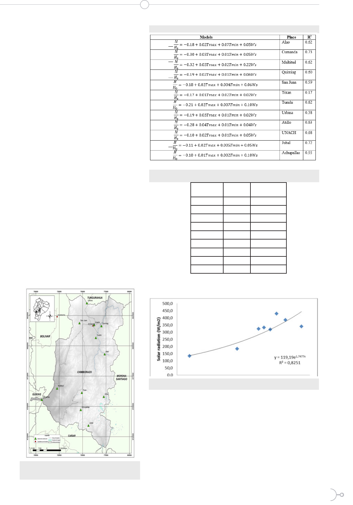
in other locations, the model proposed
by Reddy was used in other weather
stations to recover historical informa-
tion. Figure 4 shows the locations of
the weather stations. As the local condi-
tions strongly influence the atmospheric
transmissivity, individual coefficients
had to be calculated for every location.
The results are presented in table 4.
Model a b Standard
Deviation
Error Reliability r
2
Prescott 0.175 0.294 0.034 -0.013 90% - 95% 0.790
Hargreaves -0.095 0.115 0.053 0.359 94% - 95% 0.474
García 0.112 0.188 0.054 0.202 89% - 95% 0.455
Coefcient of
validation
Prescot Hargreaves García Campbell Hunt Reddy
R2 0.790 0.474 0.455 0.509 0.555 0.662
Model Dependency Relation
Bristow – Campbell Difference of temperature
.
(. )exp
H
H
t
0 469
10317
.
0
0 827
D
=
--
6@
D e m o
Hunt Difference of temperature,
Maximum temperature,
Precipitation.
.. ..ma
xm
in
H
H
tT
TP
R036014 0030002
.
0
05
D
=+ +-
D e m o
Richardson
Reddy
Minimum temperature,
maximum temperature,
precipitation, wind speed.
..
..
min max
H
H
TT Ws0170006 00
20
048
0
=- -++
D e m o
Revista Cientíca
ISSN 1390-5740
ISSN 2477-9105
11
Coefcient of
validation
Prescot Hargreaves García Campbell Hunt Reddy
R2 0.790 0.474 0.455 0.509 0.555 0.662
3.4. Models based on satellite images
As the measurement of solar radiation
just began in January 2014, as an exam-
ple of the procedure, one correlation was
calculated using that month.
It is important to mention that not all the
stations have to be used for the correla-
tion. First, it is mandatory to eliminate
the stations whose NDVI is false. For
example, the station with the name “Es-
poch” cannot be taken into account be-
cause this station is located on concrete
floor. This means that the NDVI of the
exact location where the station is pla-
ced have a very low NDVI value, which
is completely unrelated to the solar ra-
diation of that place.
Table 5 shows the data used for the
calculation of the correlation (includes
“Espoch” station to demonstrated how
unrelated are NDVI and solar radiation
in that case) and Figure 6. shows the plot
and correlation that was obtained.
Ramos,Pérez N,Villacreses,Vaca,Chavez,Pérez M.
Figure 4: Location of the weather stations where
the models were tested.
Figure 6. Solar radiation vs. NDVI – January 2014
Table 5. Data used for the calculation of correlation
4. DISCUSSION
According to Myers (14), Prescott recommends values of
a between 0.17 and 0.43, and for b between 0.24 and 0.75.
In addition, the values a = 0.29 and b = 0.42 were pro-
posed by Frere (15) and cited by Baigorria (2) for the all
Andean Highlands; these values are based in meteorolo-
gical data of stations in the Andean Region of Peru. In this
Table 4. Results of the model applied to other locations
Nombre NDVI Average Solar
radiation
Cumanda 0,36 183,9
Multitud 0,077 132,8
Quimiag 0,65 384,9
Espoch 0,29 406,9
Tunshi 0,60 427,6
Alao 0,53 331,3
Atillo 0,56 317,9
Tixan-Pistilli 0,49 323,1
Urbina 0,75 338,8

12
Número 16 Vol. 2 (2016)
R
eferences
work, for the model of Prescott, the obtained values are
in the range of those proposed by Prescott. On the other
hand, in comparison with the values proposed by Frere,
the coefcients of this work are lower because the cloudi-
ness in the Ecuadorian Andean region is more severe than
the one found in the Andean region of Peru.
For the models based on the difference of temperatures, it
is not possible to make a fair comparison because each re-
gion has particular meteorological conditions which affect
the temperatures reached. Even if the cities have similar
altitudes, the values presented by Baigorria for different
cities in the Andean Region of Peru cannot be compared
since the latitudes of the places are different.
Also, the coefcients calculated for the variable “preci-
pitation” in the models of Hunt and Reddy are close to
zero, which is an indication that this variable is irrelevant
and it does not have inuence in the estimation of the so-
lar radiation. On the contrary, the incorporation of the va-
riable “wind speed” in the model of Reddy improves the
r
2
, which is logic because the presence of wind a direct
consequence of the interaction of solar radiation with at-
mosphere.
By looking at the results of using the model proposed by
Reddy, it is clear that this model can be used safely used
in other locations. The r
2
shown in table 3 for this model
is 0.662, and comparing his value with those shown in
table 4, it can be seen that they are around the same value,
except for “Tixan”, where the correlation is low.
On the other hand, the simple relation between monthly
average solar radiation and NDVI has a high mathemati-
cal agreement. However, it is important not to forget that
NDVI is inuenced by many factors and that this method
should be used only for preliminary estimations.
5. CONCLUSIONS
In summary, it had been demonstrated in
this work that the best model to estimate
the solar radiation based on other meteo-
rological variables is the use of the suns-
hine hours. In addition, it is clear that a
multivariate analysis is capital to detect,
and separate the outliers to improve the
estimation of the solar radiation with any
model.
Moreover, it is clear that every region
has particular meteorological conditions,
which means that extrapolate the results
of one region to estimate the radiation in
other region may not be adequate, even if
both regions share some characteristics
such to be located in the Andean Region
or to have similar altitudes.
Finally, the coefcient of correlation
is high enough in some models to
allow using their empirical coefcients
to complete historical missing data of
solar radiation in the Ecuadorian Andean
region, so that researchers can use safely
the values of solar radiation for their fu-
ture work. In the case of using NDVI,
every correlation should be calculated
for every month, with their specic
set of data to be able to extrapolate to
other locations, and only if eld informa-
tion is not available to use other models.
6. ACKNOWLEDGMENTS
The authors would like to thank to Se-
cretaría de Educación Superior, Ciencia,
Tecnología e Innovación (SENESCYT)
for his nancial support to perform this
work.
(1) Fauconnier C, Haesbroeck G. Outliers detection with the minimum covariance determinant
estimator in practice. Statistical Methodology. 2009 Jul 31;6(4):363-79.
(2) Baigorria GA, Villegas EB, Trebejo I, Carlos JF, Quiroz R. Atmospheric transmissivity: dis-
tribution and empirical estimation around the central Andes. International Journal of Climatology.
2004 Jul 1;24(9):1121-36.
(3) Dufe JA, Beckman WA. Solar engineering of thermal processes. New York: Wiley; 2013
Apr 3.
(4) Tolabi HB, Moradi MH, Ayob SB. A review on classication and comparison of different mo-
Revista Cientíca
ISSN 1390-5740
ISSN 2477-9105

13
(4) Tolabi HB, Moradi MH, Ayob SB. A review on classication and comparison of different mo-
dels in solar radiation estimation. International Journal of Energy Research. 2014 May 1;38(6):689-
701.
(5) Peña D. Análisis de datos multivariantes. Madrid: McGraw-Hill; 2002.
(6) Cook RD, Hawkins DM. Unmasking multivariate outliers and leverage points: comment.
Journal of the American Statistical Association. 1990 Sep 1;85(411):640-4.
(7) Iqbal M. An introduction to solar radiation. Elsevier; 2012 Dec 2.
(8) Şahin AD. A new formulation for solar irradiation and sunshine duration estimation. Inter-
national Journal of Energy Research. 2007 Feb 1;31(2):109-18.
(9) Myers DR. Solar radiation modeling and measurements for renewable energy applications:
data and model quality. Energy. 2005 Jul 31;30(9):1517-31.
(10) Almorox J. Estimating global solar radiation from common meteorological data in Aran-
juez, Spain. Turkish Journal of Physics. 2011 Apr 12;35(1):53-64.
(11) NASA. (2014). Earth Science Oce. Retrieved from http://weather.msfc.nasa.gov/GOES/
(12) NASA 2. (2014). MODIS Characterization Support Team. Retrieved from http://mcst.gsfc.
nasa.gov/
(13) Verdin J, Pedreros D, Eilerts G. Índice Diferencial de Vegetación Normalizado (NDVI).
FEWS-Red de Alerta Temprana Contra la Inseguridad Alimentaria, Centroamérica, USGS/EROS
Data Center. 2003.
(14) Myers DR. Solar radiation: practical modeling for renewable energy applications. CRC
Press; 2013 Mar 4.
(15) Frère M, Rea J, Rijks JQ. Proyecto Interinstitucional en agroclimatología. Estudio agrocli-
matológico de la zona andina: Informe técnico.